1. PAT as a forward model

2. PAT as a inverse problem
     Backpropagation   Tikhonov regularization  Iterative regularization  Find 𝛼 and 𝑝  Iterative regularization (continuation)  Example: finding the system matrix 

3. Current applications

4. References

Photoacoustic Tomography (PAT) is a biomedical imaging technique which takes advantage of optical absorption in tissue. In the photoacoustic effect a nanosecond pulsed laser fires light onto a biological sample. Light is absorbed by the sample generating a temperature rise which will produce an initial photoacoustic pressure generating an acoustic wave. In order to detect the ultrasonic emission, we can set an array of ultrasound transducers surrounding the sample. The main advantage of PAT is that thicker tissue can be imaged as the mean free path of an acoustic wave is two or three orders of magnitude higher than an optical wave. Thus, the acoustic scattering is lesser than optical scattering and waves are less attenuated. In summary: PAT gives us optical contrast with ultrasound resolution in deep tissue. Resolution and contrast are key terms in biomedical imaging

techniques. Regarding PAT, spatial resolution depends on the relation between electromagnetic pulse duration τ and thermal

diffusion given by: where is the targeted spatial resolution and is the thermal diffusivity constant in tissue. This condition is known as thermal confinement. Moreover, contrast depends upon the

optical radiation fluence rate and the absorption coefficient of the sample. Obviously, the higher absorption coefficient, the stronger Photoacoustic (PA) wave. There is a non-linear relationship between the strength of laser radiation and the obtained PA wave. Higher fluence might burn the sample. However, below this threshold we consider the amount of generated heat by tissue as a linear process. Nevertheless, there is a tradeoff between sample thickness and resolution. In thick samples, higher frequencies (related to small features/details) will be attenuated more than in a thinner sample. Structures larger than the thermal confinement threshold will not be resolved. Comparing PAT to conventional ultrasound imaging, ultrasound is based on pulsed-echo imaging where the ultrasound wave is generated outside the sample and scattered back to the transducer. In photoacoustic the wave is generated inside the sample using the mentioned laser pulse,it is applicable to nondestructive materials that have low contrast in conventional ultrasound imaging. ^[1]

PAT as a forward model

Given an arbitrary sample and an array of transducers surrounding it, the pressure detected at can be expressed in the frequency domain as:

, (1)

where is the volume of the arbitrary source and is the expression of the impulse response modeled as a spherical wave going outwards.^[2]

PAT as a inverse problem

Backpropagation

Similar to X-ray CT, PAT is a multidimensional inverse problem where the challenge is to estimate the absorbed optical energy in tissue from a finite number of projections given by the array of transducers. The mathematical basis was set by Johann Radon, a spherical Radon transform is used in PAT. The back-projection formula is given by:

, (2)

where is the Green's function modeled by a spherical wave going inwards, is the normal of traducer's surface pointing to the sample and denotes the gradient over variable .The previous equation works for planar, cylindrical and spherical transducer geometries. Backprojection is a robust method in PAT but as it can be seen it does not provide

quantitative results, existence of streaking artifacts, nonphysical values (negative pressure does not exist) and we need a high number of ultrasound transducers in order to resolve high frequencies or small details To overcome these limitations a wide range of model-based inversion algorithms have been proposed. For instance, if we want to consider multiple wavelengths we will need some algorithm that outputs a quantitative result to see how does different spectra interact with the tissue.

Tikhonov regularization

Tikhonov regularization is the most used algorithm to solve ill-posed inverse problems. In PAT, the purpose is to minimize a cost function with respect to the absorbed optical energy in tissue:

, (3)

where is the expression, is the system matrix or impulse response, is the regularization parameter and is the pressure distribution in the transducers. In order to model a priori information is considered. Depending on the considerations for each PAT configuration the system matrix is created in a different way and it is valid for any samples. ^[3] For instance, some papers consider attenuation in media, different transducers configuration, change the number of elements in the array, non-ideal frequency response or perfect scenarios.

The remaining question is how to choose the correct regularization parameter. There is no perfect way to do it, it will depend on the system. However, there are common algorithms that will lead to best approximation such as Generalized cross-validation (GCV) , LSQR ^[4] or L-curve which do not require any prior information as discrepancy principle.

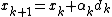
Iterative regularization

The main purpose of iterative algorithms in inverse problems is to regularize a solution of an ill-posed problems by being closer to the minimum at each iteration (convergence). The conjugate gradient (CG) is an iterative regularization method used for solving sparse systems and LSQR is analytically equivalent to CG but possessing more favorable numerical properties. CG is based on the gradient descent where a quadratic function is minimized (or a linear system). An initial guess is chosen, arbitrarily. Then, compute the negative gradient of at the initial guess since that is the direction of the decreasing values and find the minimum along the gradient line. Many methods can do this, such as Newton’s method. The obtained minimum is now the next guess, note that the next gradient must be orthogonal to the previous one. By doing this iteratively the minimum is found. However, this process might require many iterations. This is when conjugate gradients are introduced.

Given an dimensional feature space, in the conjugate gradient method the point is to search along conjugate direction such that progress made in one direction does not affect progress made in the other directions. Thus, the number of iterations will be . Conjugate vectors are defined by: In other words, 𝑢 and 𝑣 are conjugate with respect to some matrix 𝐴 the inner product is 0, also known as A-orthogonal. Having a set of 𝑛 mutually conjugate vectors means that a basis for can be formed and the solution to the linear system can be expressed as a linear combination of the vectors and some coefficients: (4) where are the coefficients and the conjugate vectors.

Find 𝛼 and 𝑝

By left-multiplying both sides of equation 4 by , 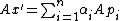, and it is known that (linear system). If both sides of the equation are now left-multiplied by an arbitrary conjugate vector , . Since and are A-orthogonal and solving for the coefficients are given by: . Now the conjugate vectors can be found by utilizing the eigenvalue problem However, it is more efficient to generate the conjugate vectors dynamically by taking a first guess and calculating its negative gradient as the first orthogonal vector and compute the first coefficient as . Then . The next conjugate vector will be . Generalizing:

; ^[5]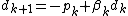

where .

Iterative regularization (continuation)

There are other ways to implement gradient descent in order to solve fast or real-time problems in photoacoustics. For instance, total variation gradient descent (TV-GD for sparse-view reconstruction. Total variation is based on CS theory which claims that the signal is sparse in a certain domain (Fourier

domain, wavelet domain, etc.) and by minimizing the 𝑙1 −𝑛𝑜𝑟𝑚 in such domain the signal can be recovered from less a

priori knowledge. ^[6] The algorithm can be summarized as (i) discretize the obtained pressure in the US

transducers and calculate the system matrix 𝐴. (ii) Iteration: the gradient descent method. The reconstructed image is the smallest TV value, so the reconstruction turns into an

optimization problem. (iii) Update or stop until the error meets some stated threshold. As PAT is sensitive to boundaries due to optical absorption, computing its finite difference can lead into a PAT sparse representation that might not exist in the spatial domain. For instance, if we want to increase the imaging speed in PAT we can make use of CS. The number of measurements can be reduced: instead of sampling point-wise we could take linear measurements, which implies that we need to find a basis to form a linear combination of the recovered pressure. Suppose that a suitable basis is found, orthonormal wavelets, representing sparse pressure. Then, apply our inverse problem solving method and the initial optical absorbed energy is recovered.

Moreover, improvements to CG have been done, LSQR ^[7] is an algorithm with similar style to CG. The matrix 𝐴 is used only to compute products of the form 𝐴𝑣 and 𝐴 𝑇𝑢 – where 𝑢 and v are vectors and generating a sequence of approximations such that the cost function is decreased monotonically. LSQR is mainly

based on the Golub & Kahan bidiagonalization and Lanczos process. It is more advantageous to solve the least squares problem using standard QR decomposition of a bidiagonal matrix. There are also current methods that are faster than LSQR, such as LSMR.

Example: finding the system matrix

There are multiple ways to find the system matrix in simulations. ^[8] One of the simplest ones, specially when computation time is a problem is the following: consider a medium with no attenuation and an ideal frequency response of the transducers to a given impulse. An imaging region can be defined inside the transducer array,^[9] the size of the region depends upon the available processing memory. For instance, a matrix of 100x100 will have 10000 different impulse responses taking into account that PAT is a spatial variant system. On the other hand the number of rows will depend on the number of time steps taken in the simulation. Then the final system matrix will contain: [number of steps x number of transducers, points in the imaging region]. The only difference between the impulse response between in such points is a time delay between transducers as we had previously considered an ideal medium and response. By considering attenuating medium there are other techniques to compute the system matrix by using Singular Value Decomposition (SVD).

Current applications

Current papers in PAT reconstruction are following the same trend as the last decade: improving the accuracy and the speed. For instance using the previously mentioned Lanczos bidiagonalization to make the system computationally efficient. Then, the minimization of the cost function by Tikhonov regularization is performed by extrapolating the object at multiple values of the regularization parameter. Thus, the extrapolation avoids evaluating the regularization parameter automatically (computationally demanding). An interpolated model-matrix inversion ^[10] increases the accuracy of an optoacoustic system. Interpolation can be performed by tiling the x-y reconstruction plane with right-angle triangles with vertexes on the grid point. Normally the increase on accuracy would lead into slow algorithms but this problem can be solved using interpolation plus LSQR. Furthermore, the SVD can be used to analyze PAT systems and solve inverse problems, laser-induced noise ^[11] can be removed from photoacoustic images. During raw radiofrequency acquisition noise is acquired in multiple transducer elements - induced by the nanosecond laser pulse. The singular value decomposition of acquired radiofrequency data matrix 𝑋 is computed. The estimation of the laser induced noise relies on the singular value components. Only the largest value components are retained (truncated SVD). It turns out that there is dependency of the signal amplitude and the retained singular value components after the truncation which is used to apply the noise removal.

References

• Mildenhall photographic collection
• Mildenhall railway station
• Mildenhall Road railway station
• Mildenhall Town
• Mildenhall Town F.C.
• Mildenitz
• Mildert
• Mild hybrid
• Mild Hybrid
• Mil (disambiguation)
• Mildly context-sensitive language
• Mildly context sensitive language
• Mild malt
• Mildmay
• Mildmay Fane, 2nd Earl of Westmorland
• Mildmay Monarchs
• Mildmay, Ontario
• Mildmay Park railway station
• Mild mental retardation
• Mildred
• Mildred A. Babb
• Mildred Aldrich
• Mildred Ames
• Mildred and Richard Loving
• Mildred Anne Butler