“Draft:Quasi-Eulerian mean velocity”的意思、由来-开放百科全书

词条

Draft:Quasi-Eulerian mean velocity

释义

The Generalized Lagrangian Mean velocity
Quasi-Eulerian mean velocity
References
External links

{{AFC submission|d|v|u=Duoc Nguyen|ns=118|decliner=Scope creep|declinets=20181121222613|ts=20181015223714}} {{AFC comment|1=No inline citations. Please check REFB for help in forming inline citations.

Also the article had no lede. Please form a lede, reference and resubmit. Article is also not linked. scope_creep (talk) 22:26, 21 November 2018 (UTC)}}

The Generalized Lagrangian Mean velocity

In fluid mechanics, the Reynolds-averaged Navier-Stokes equations (RANS) are usually employed to calculate the mean motion of the fluid flow. The RANS equations are given in Eulerian mean framework, in which the variables are defined at fixed positions in the spatial space. The solution of these equations gives the Eulerian mean velocity. However, the region between the wave trough and the wave crest is not always filled by the fluid. In a part of the wave period this region is filled by the air. Because of the big different in density between the air and the fluid then the use of RANS equations in this area poses problem (Ardhuin et al., 2008).

The above problem can be solved by Generalized Lagrangian mean (GLM) method, which was proposed by Andrews & McIntyre (1978). The basic idea of this method is averaging over disturbance positions of fluid particle. The GLM velocity is defined by:

In the above, the overbar notation expresses the time average, is the position, t is the time, is called the GLM velocity, and expresses the disturbance displacement of the fluid particle. The GLM method is valid from the water bottom to the mean surface water level even in condition of finite amplitude surface wave.

Quasi-Eulerian mean velocity

A set of equations of motion of fluid particle written in term of GLM velocity was developed by Andrews & McIntyre (1978). However, in this set of equations, the effect of the wave and turbulence on the mean current is still implicit. Therefore, they are only applicable for non-turbulent motion and where the linear wave theory is valid.

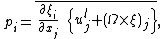
An effective method to solve the GLM equations are rewritten them in term of quasi-Eulerian mean velocity. This method was employed by Ardhuin et al. (2008) to develop an explicit wave-average equations using GLM method. In which, they used hypotheses of weak horizontal gradients of the mean current and water depth, small surface slope, and weak curvature of the mean current profile. The quasi-Eulerian mean velocity in i^th direction is defined by:

where, is the quasi-Eulerian mean velocity, and is the pseudo-momentum defined by:

in which, the Einstein notation or Einstein summation convention is employed with the index j run over the set {1, 2, 3},

is the angular velocity of the Earth, and is the Lagrangian disturbance velocity defined by:

According to Andrews & McIntyre (1978), the pseudo-momentum is approximated to Stokes drift when the surface wave is irrotational and the mean current is of second order of the wave amplitude. In general, we do not have such relationship. Therefore, the equations of Ardhuin et al. (2008) are probably accurate for ocean mixed layer and shoaling waves. For surf zone applications, it only gives qualitative results.

Bennis et al. (2011) developed the equations of Ardhuin et al. (2008) for coastal applications. In this, the forcing which is caused by breaking wave, wave-induced mixing, and bottom friction are included. Moreover, in their work, the quasi-Eulerian mean velocity is defined based on the definition of Jenkins (1989), i.e.:

where, is the Stokes drift. This is a better approximation for the Eulerian mean velocity, especially for coastal areas where rotation effects of the waves are significant. Similar to GLM velocity, the quasi-Eulerian mean velocity is valid from the water bottom to the mean water surface level.

The quasi-Eulerian mean equations of motion of Bennis et al. (2011) have been applied widely in numerical ocean models such as MARS3D model, SYMPHONIE model, and TELEMAC-3D model.

References

Andrews, D. G., & McIntyre, M. E. (1978). An exact theory of nonlinear waves on a Lagrangian-mean flow. Journal of Fluid Mechanics, 89(4), 609-646.
Ardhuin, F., Rascle, N., & Belibassakis, K. A. (2008). Explicit wave-averaged primitive equations using a generalized Lagrangian mean. Ocean Modelling, 20(1), 35-60.
Bennis, A.-C., Ardhuin, F., & Dumas, F. (2011). On the coupling of wave and three-dimensional circulation models: Choice of theoretical framework, practical implementation and adiabatic tests. Ocean Modelling, 40(3), 260-272.
Jenkins, A. D. (1989). The use of a wave prediction model for driving a near-surface current model. Deutsche Hydrografische Zeitschrift, 42(3-6), 133-149.

External links

www.example.com

随便看

开放百科全书收录14589846条英语、德语、日语等多语种百科知识，基本涵盖了大多数领域的百科知识，是一部内容自由、开放的电子版国际百科全书。