色立体
表示色彩标准系统的立体模型,以色彩三属性为骨架有规律地组织安排各种色彩。
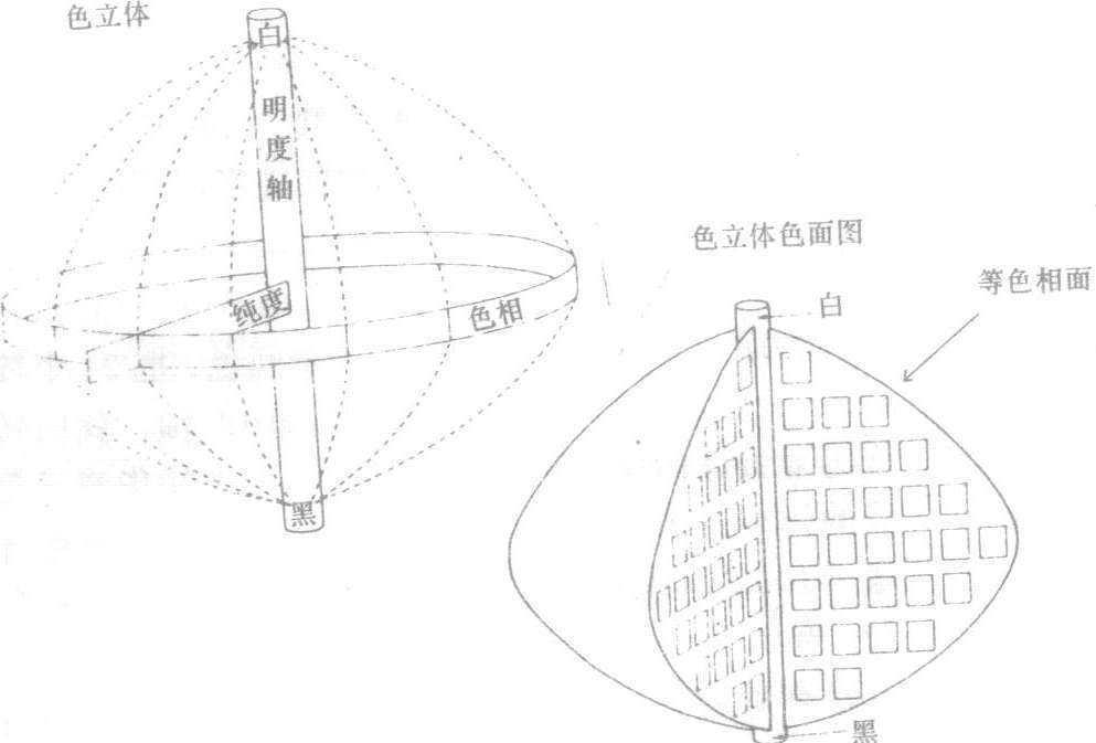
色立体Seliti
用一个三维空间的立体形可以把颜色的三种基本特性:明度、色相、纯度全部表示出来。在色立体中,垂直轴代表白黑系列明度的变化,顶端是白色,底端是黑色,中间是各种灰色的过渡。色相由水平面的圆周表示,圆周上的各点代表各种不同的色相,圆形的中心是中灰色,中灰色的明度和圆周上各种色相的明度相同,从圆周向圆心过渡,表示颜色的纯度逐渐降低,从圆周向上下白黑方向的变化,也表示颜色纯度的降低。颜色色相和纯度的改变,不一定伴随明度的变化,当颜色在色立体同一平面上变化时,只改变色相和纯度,而不改变明度,但只要颜色离开了圆周,就不再是最饱和的颜色了。色立体是理想化了的示意模型,目地是为了使人更容易理解色彩的三属性之间的关系。
色立体