“Tridiagonal matrix algorithm”的意思、由来-开放百科全书

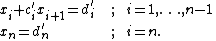
In numerical linear algebra, the tridiagonal matrix algorithm, also known as the Thomas algorithm (named after Llewellyn Thomas), is a simplified form of Gaussian elimination that can be used to solve tridiagonal systems of equations. A tridiagonal system for n unknowns may be written as

For such systems, the solution can be obtained in

operations instead of

required by Gaussian elimination. A first sweep eliminates the

's, and then an (abbreviated) backward substitution produces the solution. Examples of such matrices commonly arise from the discretization of 1D Poisson equation and natural cubic spline interpolation.

Thomas' algorithm is not stable in general, but is so in several special cases, such as when the matrix is diagonally dominant (either by rows or columns) or symmetric positive definite;^[1]^[2] for a more precise characterization of stability of Thomas' algorithm, see Higham Theorem 9.12.^[2] If stability is required in the general case, Gaussian elimination with partial pivoting (GEPP) is recommended instead.^[3]

Method

The forward sweep consists of modifying the coefficients as follows, denoting the new coefficients with primes:

The method above preserves the original coefficient vectors. If this is not required, then a much simpler form of the algorithm is

The implementation in a VBA subroutine without preserving the coefficient vectors is shown below

Derivation

The derivation of the tridiagonal matrix algorithm is a special case of Gaussian elimination.

where the second equation immediately above is a simplified version of the equation immediately preceding it. The effect is that

has been eliminated from the second equation. Using a similar tactic with the modified second equation on the third equation yields:

This time

was eliminated. If this procedure is repeated until the

row; the (modified)

equation will involve only one unknown,

. This may be solved for and then used to solve the

equation, and so on until all of the unknowns are solved for.

Clearly, the coefficients on the modified equations get more and more complicated if stated explicitly. By examining the procedure, the modified coefficients (notated with tildes) may instead be defined recursively:

To further hasten the solution process,

may be divided out (if there's no division by zero risk), the newer modified coefficients, each notated with a prime, will be:

This gives the following system with the same unknowns and coefficients defined in terms of the original ones above:

The last equation involves only one unknown. Solving it in turn reduces the next last equation to one unknown, so that this backward substitution can be used to find all of the unknowns:

Variants

In some situations, particularly those involving periodic boundary conditions, a slightly perturbed form of the tridiagonal system may need to be solved:

In this case, we can make use of the Sherman-Morrison formula to avoid the additional operations of Gaussian elimination and still use the Thomas algorithm. The method requires solving a modified non-cyclic version of the system for both the input and a sparse corrective vector, and then combining the solutions. This can be done efficiently if both solutions are computed at once, as the forward portion of the pure tridiagonal matrix algorithm can be shared.

In other situations, the system of equations may be block tridiagonal (see block matrix), with smaller submatrices arranged as the individual elements in the above matrix system (e.g., the 2D Poisson problem). Simplified forms of Gaussian elimination have been developed for these situations.^[4]

The textbook Numerical Mathematics by Quarteroni, Sacco and Saleri, lists a modified version of the algorithm which avoids some of the divisions (using instead multiplications), which is beneficial on some computer architectures.

Parallel tridiagonal solvers have been published for many vector and parallel architectures, including GPUs^[5]

For an extensive treatment of parallel tridiagonal and block tridiagonal solvers see ^[7]

References

1. ^{{cite book|author=Pradip Niyogi|title=Introduction to Computational Fluid Dynamics|year=2006|publisher=Pearson Education India|isbn=978-81-7758-764-7|page=76}}
2. ^{{cite book|author=Nicholas J. Higham|title=Accuracy and Stability of Numerical Algorithms: Second Edition|year=2002|publisher=SIAM|isbn=978-0-89871-802-7|page=175}}
3. ^¹{{cite book|author=Biswa Nath Datta|title=Numerical Linear Algebra and Applications, Second Edition|year=2010|publisher=SIAM|isbn=978-0-89871-765-5|page=162}}
4. ^{{cite book|last1=Quarteroni|first1=Alfio|last2=Sacco|first2=Riccardo|last3=Saleri|first3=Fausto | year=2007|title=Numerical Mathematics|publisher= Springer, New York|isbn= 978-3-540-34658-6|chapter=Section 3.8}}
5. ^{{cite conference|last1=Chang|first1=L.-W.|last2=Hwu|first2=W,-M.|title=A guide for implementing tridiagonal solvers on GPUs|book-title=Numerical Computations with GPUs|publisher=Springer|isbn=978-3-319-06548-9|editor=V. Kidratenko|year=2014}}
6. ^{{cite article|last1=Venetis|first1=I.E.|last2=Kouris|first2=A.|last3=Sobczyk|first3=A.|last4=Gallopoulos|first4=E.|last5=Sameh|first5=A.|title=A direct tridiagonal solver based on Givens rotations for GPU architectures|journal=Parallel Computing|volume=49|pages=101-116|year=2015}}
7. ^{{cite book|last1=Gallopoulos|first1=E.|last2=Philippe|first2=B.|last3=Sameh|first3=A.H. | year=2016|title=Parallelism in Matrix Computations|publisher= Springer|isbn= 978-94-017-7188-7|chapter=Chapter 5}}