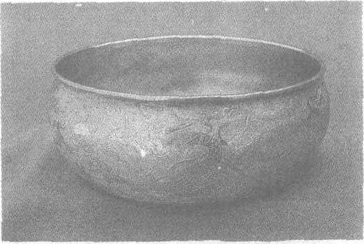
请输入您要查询的百科知识:


词条 Geometric distribution
释义

  1. Introduction to the geometric distribution

     Examples  Assumptions: When is the geometric distribution an appropriate model?  Probability of outcomes  Expected number of failures before the first success  

  2. Moments and cumulants

  3. Parameter estimation

  4. Other properties

  5. Related distributions

  6. Computer software for the geometric distribution

     Geometric distribution using R  Geometric distribution using Excel 

  7. See also

  8. References

  9. External links

{{Infobox probability distribution 2
| name = Geometric
| type = mass
| pdf_image =
| cdf_image =
| parameters = success probability (real)
| support = k trials where
| pdf =
| cdf =
| mean =
| median =

(not unique if is an integer)


| mode =
| variance =
| skewness =
| kurtosis =
| entropy =
| mgf =
for
| char =
| parameters2 = success probability (real)
| support2 = k failures where
| pdf2 =
| cdf2 =
| mean2 =
| median2 =

(not unique if is an integer)


| mode2 =
| variance2 =
| skewness2 =
| kurtosis2 =
| entropy2 =
| mgf2 =
| char2 =
}}

In probability theory and statistics, the geometric distribution is either of two discrete probability distributions:

  • The probability distribution of the number X of Bernoulli trials needed to get one success, supported on the set { 1, 2, 3, ...}
  • The probability distribution of the number Y = X − 1 of failures before the first success, supported on the set { 0, 1, 2, 3, ... }

Which of these one calls "the" geometric distribution is a matter of convention and convenience.

These two different geometric distributions should not be confused with each other. Often, the name shifted geometric distribution is adopted for the former one (distribution of the number X); however, to avoid ambiguity, it is considered wise to indicate which is intended, by mentioning the support explicitly.

The geometric distribution gives the probability that the first occurrence of success requires k independent trials, each with success probability p. If the probability of success on each trial is p, then the probability that the kth trial (out of k trials) is the first success is

for k = 1, 2, 3, ....

The above form of the geometric distribution is used for modeling the number of trials up to and including the first success. By contrast, the following form of the geometric distribution is used for modeling the number of failures until the first success:

for k = 0, 1, 2, 3, ....

In either case, the sequence of probabilities is a geometric sequence.

For example, suppose an ordinary die is thrown repeatedly until the first time a "1" appears. The probability distribution of the number of times it is thrown is supported on the infinite set { 1, 2, 3, ... } and is a geometric distribution with p = 1/6.

Introduction to the geometric distribution

Consider a sequence of trials, where each trial has only two possible outcomes (designated failure and success). The probability of success is assumed to be the same for each trial. In such a sequence of trials, the geometric distribution is useful to model the number of failures before the first success. The distribution gives the probability that there are zero failures before the first success, one failure before the first success, two failures before the first success, and so on.

Examples

A newlywed couple plans to have children, and will continue until the first girl. What is the probability that there are zero boys before the first girl, one boy before the first girl, two boys before the first girl, and so on?

A doctor is seeking an anti-depressant for a newly diagnosed patient. Suppose that, of the available anti-depressant drugs, the probability that any particular drug will be effective for a particular patient is p=0.6. What is the probability that the first drug found to be effective for this patient is the first drug tried, the second drug tried, and so on? What is the expected number of drugs that will be tried to find one that is effective?

A patient is waiting for a suitable matching kidney donor for a transplant. If the probability that a randomly selected donor is a suitable match is p=0.1, what is the expected number of donors who will be tested before a matching donor is found?

Assumptions: When is the geometric distribution an appropriate model?

The geometric distribution is an appropriate model if the following assumptions are true.

  • The phenomenon being modelled is a sequence of independent trials.
  • There are only two possible outcomes for each trial, often designated success or failure.
  • The probability of success, p, is the same for every trial.

If these conditions are true, then the geometric random variable is the count of the number of failures before the first success. The possible number of failures before the first success is 0, 1, 2, 3, and so on. The geometric random variable Y is the number of failures before the first success. In the graphs above, this formulation is shown on the right.

An alternative formulation is that the geometric random variable X is the total number of trials up to and including the first success, and the number of failures is X-1. In the graphs above, this formulation is shown on the left.

Probability of outcomes

Consider the anti-depressant example above. The probability that any given drug is effective (success) is p = 0.6. The probability that a drug will not be effective (fail) is q = 1 – p = 1 – 0.6 = 0.4. Here are probabilities of some possible outcomes.

(i) The first drug works. There are zero failures before the first success. Y = 0 failures. The probability P(zero failures before first success) is simply the probability that the first drug works.

(ii) The first drug fails, but the second drug works. There is one failure before the first success. Y= 1 failure. The probability for this sequence of events is p(first drug fails) p(second drug is success) which is given by

(iii) The first drug fails, the second drug fails, but the third drug works. There are two failures before the first success. Y= 2 failures. The probability for this sequence of events is p(first drug fails) p(second drug fails) p(third drug is success)

The general formula to calculate the probability of k failures before the first success, where the probability of success is p and the probability of failure is q = 1 − p, is

for k = 0, 1, 2, 3, ....

For the newlyweds awaiting their first girl, the probability of no boys before the first girl is

The probability of one boy before the first girl is

The probability of two boys before the first girl is

and so on.

Expected number of failures before the first success

For the geometric distribution, the expected (mean) number of failures before the first success is E(Y) = (1 − p)/p.

For the anti-depressant example, with p = 0.6, the mean number of failures before the first success is E(Y) = (1 − p)/p = (1 − 0.6)/0.6 = 0.67.

For the kidney-donor example, with p = 0.1, the mean number of failures before the first success is E(Y) = (1 − 0.1)/0.1 = 9.

For the alternative formulation, where X is the number of trials up to and including the first success, the expected value is E(X) = 1/p.

Moments and cumulants

The expected value of a geometrically distributed random variable X is 1/p and the variance is (1 − p)/p2:

Similarly, the expected value of the geometrically distributed random variable Y = X − 1 (where Y corresponds to the pmf listed in the right column) is q/p = (1 − p)/p, and its variance is (1 − p)/p2:

Let μ = (1 − p)/p be the expected value of Y. Then the cumulants of the probability distribution of Y satisfy the recursion

Outline of proof: That the expected value is (1 − p)/p can be shown in the following way. Let Y be as above. Then

(The interchange of summation and differentiation is justified by the fact that convergent power series converge uniformly on compact subsets of the set of points where they converge.)

Parameter estimation

For both variants of the geometric distribution, the parameter p can be estimated by equating the expected value with the sample mean. This is the method of moments, which in this case happens to yield maximum likelihood estimates of p.{{citation needed|date=May 2012}}

Specifically, for the first variant let k = k1, ..., kn be a sample where ki ≥ 1 for i = 1, ..., n. Then p can be estimated as

In Bayesian inference, the Beta distribution is the conjugate prior distribution for the parameter p. If this parameter is given a Beta(αβ) prior, then the posterior distribution is{{citation needed|date=May 2012}}

The posterior mean E[p] approaches the maximum likelihood estimate as α and β approach zero.

In the alternative case, let k1, ..., kn be a sample where ki ≥ 0 for i = 1, ..., n. Then p can be estimated as

The posterior distribution of p given a Beta(αβ) prior is{{citation needed|date=May 2012}}

Again the posterior mean E[p] approaches the maximum likelihood estimate as α and β approach zero.

Other properties

  • The probability-generating functions of X and Y are, respectively,

  • Like its continuous analogue (the exponential distribution), the geometric distribution is memoryless. That means that if you intend to repeat an experiment until the first success, then, given that the first success has not yet occurred, the conditional probability distribution of the number of additional trials does not depend on how many failures have been observed. The die one throws or the coin one tosses does not have a "memory" of these failures. The geometric distribution is the only memoryless discrete distribution.
  • Among all discrete probability distributions supported on {1, 2, 3, ... } with given expected value μ, the geometric distribution X with parameter p = 1/μ is the one with the largest entropy.{{citation needed|date=May 2012}}
  • The geometric distribution of the number Y of failures before the first success is infinitely divisible, i.e., for any positive integer n, there exist independent identically distributed random variables Y1, ..., Yn whose sum has the same distribution that Y has. These will not be geometrically distributed unless n = 1; they follow a negative binomial distribution.
  • The decimal digits of the geometrically distributed random variable Y are a sequence of independent (and not identically distributed) random variables.{{citation needed|date=May 2012}} For example, the hundreds digit D has this probability distribution:

where q = 1 − p, and similarly for the other digits, and, more generally, similarly for numeral systems with other bases than 10. When the base is 2, this shows that a geometrically distributed random variable can be written as a sum of independent random variables whose probability distributions are indecomposable.

  • Golomb coding is the optimal prefix code{{clarify|date=May 2012}} for the geometric discrete distribution.{{citation needed|date=May 2012}}

Related distributions

  • The geometric distribution Y is a special case of the negative binomial distribution, with r = 1. More generally, if Y1, ..., Yr are independent geometrically distributed variables with parameter p, then the sum

follows a negative binomial distribution with parameters r and p.[1]

  • The geometric distribution is a special case of discrete compound Poisson distribution.
  • If Y1, ..., Yr are independent geometrically distributed variables (with possibly different success parameters pm), then their minimum

is also geometrically distributed, with parameter {{citation needed|date=May 2012}}

  • Suppose 0 < r < 1, and for k = 1, 2, 3, ... the random variable Xk has a Poisson distribution with expected value r k/k. Then

has a geometric distribution taking values in the set {0, 1, 2, ...}, with expected value r/(1 − r).{{citation needed|date=May 2012}}

  • The exponential distribution is the continuous analogue of the geometric distribution. If X is an exponentially distributed random variable with parameter λ, then

where is the floor (or greatest integer) function, is a geometrically distributed random variable with parameter p = 1 − eλ (thus λ = −ln(1 − p)[2]) and taking values in the set {0, 1, 2, ...}. This can be used to generate geometrically distributed pseudorandom numbers by first generating exponentially distributed pseudorandom numbers from a uniform pseudorandom number generator: then is geometrically distributed with parameter , if is uniformly distributed in [0,1].

  • If p = 1/n and X is geometrically distributed with parameter p, then the distribution of X/n approaches an exponential distribution with expected value 1 as n → ∞, since

Computer software for the geometric distribution

Geometric distribution using R

The R function dgeom(k, prob) calculates the probability that there are k failures before the first success, where the argument "prob" is the probability of success on each trial.

For example,

dgeom(0,0.6) = 0.6dgeom(1,0.6) = 0.24

R uses the convention that k is the number of failures, so that the number of trials up to and including the first success is k + 1.

The following R code creates a graph of the geometric distribution from Y = 0 to 10, with p = 0.6.

Y=0:10

plot(Y, dgeom(Y,0.6), type="h", ylim=c(0,1), main="Geometric distribution for p=0.6", ylab="P(Y=Y)", xlab="Y=Number of failures before first success")

Geometric distribution using Excel

The geometric distribution, for the number of failures before the first success, is a special case of the negative binomial distribution, for the number of failures before s successes.

The Excel function NEGBINOMDIST(number_f, number_s, probability_s) calculates the probability of k = number_f failures before s = number_s successes where p = probability_s is the probability of success on each trial. For the geometric distribution, let number_s = 1 success.

For example,

=NEGBINOMDIST(0, 1, 0.6) = 0.6

=NEGBINOMDIST(1, 1, 0.6) = 0.24

Like R, Excel uses the convention that k is the number of failures, so that the number of trials up to and including the first success is k + 1.

See also

  • Hypergeometric distribution
  • Coupon collector's problem
  • Compound Poisson distribution
  • Negative binomial distribution
{{More footnotes|date=March 2011}}

References

1. ^Pitman, Jim. Probability (1993 edition). Springer Publishers. pp 372.
2. ^{{cite web|url=http://www.wolframalpha.com/input/?i=inverse+p+=+1+-+e%5E-l|title=Wolfram-Alpha: Computational Knowledge Engine|website=www.wolframalpha.com}}

External links

  • {{planetmath reference|id=3456|title=Geometric distribution}}
  • Geometric distribution on MathWorld.
{{ProbDistributions|discrete-infinite}}

3 : Discrete distributions|Exponential family distributions|Infinitely divisible probability distributions

随便看


开放百科全书收录14589846条英语、德语、日语等多语种百科知识,基本涵盖了大多数领域的百科知识,是一部内容自由、开放的电子版国际百科全书。


Copyright © 2023 OENC.NET All Rights Reserved
京ICP备2021023879号 更新时间:2024/9/24 2:38:36