- Formulation
- Statement of the theorem
- Proof
- Properties of the Karhunen–Loève transform Special case: Gaussian distribution The Karhunen–Loève transform decorrelates the process The Karhunen–Loève expansion minimizes the total mean square error Explained variance The Karhunen–Loève expansion has the minimum representation entropy property
- Linear Karhunen–Loève approximations
- Non-Linear approximation in bases Non-optimality of Karhunen–Loève bases
- Principal component analysis Covariance matrix Principal component transform
- Examples The Wiener process The Brownian bridge
- Applications Applications in signal estimation and detection Detection of a known continuous signal S(t) Signal detection in white noise Signal detection in colored noise How to find k(t) Test threshold for Neyman–Pearson detector Prewhitening Detection of a Gaussian random signal in Additive white Gaussian noise (AWGN)
- See also
- Notes
- References
- External links
In the theory of stochastic processes, the Karhunen–Loève theorem (named after Kari Karhunen and Michel Loève), also known as the Kosambi–Karhunen–Loève theorem[1][2] is a representation of a stochastic process as an infinite linear combination of orthogonal functions, analogous to a Fourier series representation of a function on a bounded interval. The transformation is also known as Hotelling transform and eigenvector transform, and is closely related to principal component analysis (PCA) technique widely used in image processing and in data analysis in many fields.[3]
Stochastic processes given by infinite series of this form were first considered by Damodar Dharmananda Kosambi.[4][5] There exist many such expansions of a stochastic process: if the process is indexed over {{math|[a, b]}}, any orthonormal basis of {{math|L2([a, b])}} yields an expansion thereof in that form. The importance of the Karhunen–Loève theorem is that it yields the best such basis in the sense that it minimizes the total mean squared error.
In contrast to a Fourier series where the coefficients are fixed numbers and the expansion basis consists of sinusoidal functions (that is, sine and cosine functions), the coefficients in the Karhunen–Loève theorem are random variables and the expansion basis depends on the process. In fact, the orthogonal basis functions used in this representation are determined by the covariance function of the process. One can think that the Karhunen–Loève transform adapts to the process in order to produce the best possible basis for its expansion.
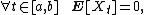
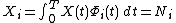
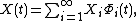
In the case of a centered stochastic process {{math|{Xt}t ∈ [a, b]}} (centered means {{math|E[Xt] {{=}} 0}} for all {{math|t ∈ [a, b]}}) satisfying a technical continuity condition, {{mvar|Xt}} admits a decomposition

where {{mvar|Zk}} are pairwise uncorrelated random variables and the functions {{mvar|ek}} are continuous real-valued functions on {{math|[a, b]}} that are pairwise orthogonal in {{math|L2([a, b])}}. It is therefore sometimes said that the expansion is bi-orthogonal since the random coefficients {{mvar|Zk}} are orthogonal in the probability space while the deterministic functions {{mvar|ek}} are orthogonal in the time domain. The general case of a process {{mvar|Xt}} that is not centered can be brought back to the case of a centered process by considering {{math|Xt − E[Xt]}} which is a centered process.
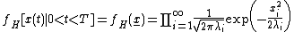
Moreover, if the process is Gaussian, then the random variables {{mvar|Zk}} are Gaussian and stochastically independent. This result generalizes the Karhunen–Loève transform. An important example of a centered real stochastic process on {{math|[0, 1]}} is the Wiener process; the Karhunen–Loève theorem can be used to provide a canonical orthogonal representation for it. In this case the expansion consists of sinusoidal functions.
The above expansion into uncorrelated random variables is also known as the Karhunen–Loève expansion or Karhunen–Loève decomposition. The empirical version (i.e., with the coefficients computed from a sample) is known as the Karhunen–Loève transform (KLT), principal component analysis, proper orthogonal decomposition (POD), empirical orthogonal functions (a term used in meteorology and geophysics), or the Hotelling transform.
Formulation
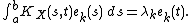
- Throughout this article, we will consider a square-integrable zero-mean random process {{mvar|Xt}} defined over a probability space {{math|(Ω, F, P)}} and indexed over a closed interval {{math|[a, b]}}, with covariance function {{math|KX(s, t)}}. We thus have:


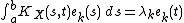
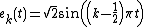
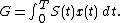
- We associate to KX a linear operator TKX defined in the following way:

Since TKX is a linear operator, it makes sense to talk about its eigenvalues λk and eigenfunctions ek, which are found solving the homogeneous Fredholm integral equation of the second kind
Statement of the theorem
Theorem. Let {{mvar|Xt}} be a zero-mean square-integrable stochastic process defined over a probability space {{math|(Ω, F, P)}} and indexed over a closed and bounded interval [a, b], with continuous covariance function KX(s, t).
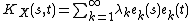
Then KX(s,t) is a Mercer kernel and letting ek be an orthonormal basis on {{math|L2([a, b])}} formed by the eigenfunctions of TKX with respective eigenvalues {{mvar|λk, Xt}} admits the following representation
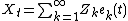
where the convergence is in L2, uniform in t and

Furthermore, the random variables Zk have zero-mean, are uncorrelated and have variance λk

Note that by generalizations of Mercer's theorem we can replace the interval [a, b] with other compact spaces C and the Lebesgue measure on [a, b] with a Borel measure whose support is C.
Proof
- The covariance function KX satisfies the definition of a Mercer kernel. By Mercer's theorem, there consequently exists a set {λk, ek(t)} of eigenvalues and eigenfunctions of TKX forming an orthonormal basis of L2([a,b]), and KX can be expressed as
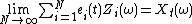
- The process Xt can be expanded in terms of the eigenfunctions ek as:
where the coefficients (random variables) Zk are given by the projection of Xt on the respective eigenfunctions
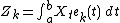
- We may then derive
where we have used the fact that the ek are eigenfunctions of TKX and are orthonormal.
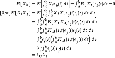
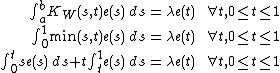
- Let us now show that the convergence is in L2. Let

Then:

which goes to 0 by Mercer's theorem.
Properties of the Karhunen–Loève transform
Special case: Gaussian distribution
Since the limit in the mean of jointly Gaussian random variables is jointly Gaussian, and jointly Gaussian random (centered) variables are independent if and only if they are orthogonal, we can also conclude:
Theorem. The variables {{mvar|Zi}} have a joint Gaussian distribution and are stochastically independent if the original process {{math|{Xt}t}} is Gaussian.
In the Gaussian case, since the variables {{mvar|Zi}} are independent, we can say more:
almost surely.
The Karhunen–Loève transform decorrelates the process
This is a consequence of the independence of the {{mvar|Zk}}.
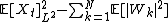
The Karhunen–Loève expansion minimizes the total mean square error
In the introduction, we mentioned that the truncated Karhunen–Loeve expansion was the best approximation of the original process in the sense that it reduces the total mean-square error resulting of its truncation. Because of this property, it is often said that the KL transform optimally compacts the energy.
More specifically, given any orthonormal basis {fk} of L2([a, b]), we may decompose the process Xt as:
where
and we may approximate Xt by the finite sum
for some integer N.
Claim. Of all such approximations, the KL approximation is the one that minimizes the total mean square error (provided we have arranged the eigenvalues in decreasing order).
Consider the error resulting from the truncation at the N-th term in the following orthonormal expansion:

The mean-square error εN2(t) can be written as:

We then integrate this last equality over [a, b]. The orthonormality of the fk yields:

The problem of minimizing the total mean-square error thus comes down to minimizing the right hand side of this equality subject to the constraint that the fk be normalized. We hence introduce {{mvar|βk}}, the Lagrangian multipliers associated with these constraints, and aim at minimizing the following function:

Differentiating with respect to fi(t) (this is a functional derivative) and setting the derivative to 0 yields:

which is satisfied in particular when
In other words, when the fk are chosen to be the eigenfunctions of TKX, hence resulting in the KL expansion.
Explained variance
An important observation is that since the random coefficients Zk of the KL expansion are uncorrelated, the Bienaymé formula asserts that the variance of Xt is simply the sum of the variances of the individual components of the sum:

Integrating over [a, b] and using the orthonormality of the ek, we obtain that the total variance of the process is:
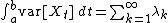
In particular, the total variance of the N-truncated approximation is

As a result, the N-truncated expansion explains

of the variance; and if we are content with an approximation that explains, say, 95% of the variance, then we just have to determine an  such that

The Karhunen–Loève expansion has the minimum representation entropy property
Given a representation of  , for some orthonormal basis
  and random
  , we let
  , so that
  . We may then define the representation entropy to be
  . Then we have
  , for all choices of
  . That is, the KL-expansion has minimal representation entropy.
Denote the coefficients obtained for the basis  as
as  , and for as
  .
.
Choose  . Note that since
  minimizes the mean squared error, we have that

Expanding the right hand size, we get:

Using the orthonormality of , and expanding  in the basis, we get that the right hand size is equal to:
We may perform indentitcal analysis for the , and so rewrite the above inequality as:
Subtracting the common first term, and dividing by  , we obtain that:

This implies that:

Linear Karhunen–Loève approximations
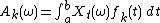
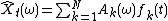
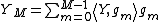
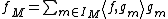
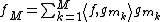
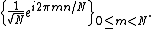
Let us consider a whole class of signals we want to approximate over the first {{mvar|M}} vectors of a basis. These signals are modeled as realizations of a random vector {{math|Y[n]}} of size {{mvar|N}}. To optimize the approximation we design a basis that minimizes the average approximation error. This section proves that optimal bases are Karhunen–Loeve bases that diagonalize the covariance matrix of {{mvar|Y}}. The random vector {{mvar|Y}} can be decomposed in an orthogonal basis

as follows:
where each
is a random variable. The approximation from the first {{math|M ≤ N}} vectors of the basis is
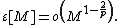
The energy conservation in an orthogonal basis implies

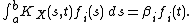
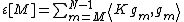
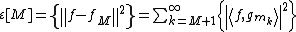
This error is related to the covariance of {{mvar|Y}} defined by
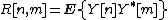
For any vector {{math|x[n]}} we denote by {{mvar|K}} the covariance operator represented by this matrix,

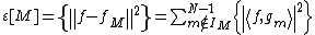
The error {{math|ε[M]}} is therefore a sum of the last {{math|N − M}} coefficients of the covariance operator
The covariance operator {{mvar|K}} is Hermitian and Positive and is thus diagonalized in an orthogonal basis called a Karhunen–Loève basis. The following theorem states that a Karhunen–Loève basis is optimal for linear approximations.
Theorem (Optimality of Karhunen–Loève basis). Let {{mvar|K}} be a covariance operator. For all {{math|M ≥ 1}}, the approximation error

is minimum if and only if

is a Karhunen–Loeve basis ordered by decreasing eigenvalues.

Non-Linear approximation in bases
Linear approximations project the signal on M vectors a priori. The approximation can be made more precise by choosing the M orthogonal vectors depending on the signal properties. This section analyzes the general performance of these non-linear approximations. A signal  is approximated with M vectors selected adaptively in an orthonormal basis for

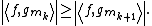
Let  be the projection of f over M vectors whose indices are in {{mvar|IM}}:
The approximation error is the sum of the remaining coefficients
To minimize this error, the indices in {{mvar|IM}} must correspond to the M vectors having the largest inner product amplitude

These are the vectors that best correlate f. They can thus be interpreted as the main features of f. The resulting error is necessarily smaller than the error of a linear approximation which selects the M approximation vectors independently of f. Let us sort

in decreasing order
The best non-linear approximation is
It can also be written as inner product thresholding:
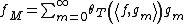
with
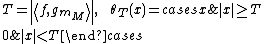
The non-linear error is
this error goes quickly to zero as M increases, if the sorted values of  have a fast decay as k increases. This decay is quantified by computing the
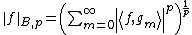
  norm of the signal inner products in B:
The following theorem relates the decay of {{math|ε[M]}} to 
Theorem (decay of error). If  with {{math|p < 2}} then
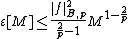
and
Conversely, if  then
then
 for any {{math|q > p}}.
Non-optimality of Karhunen–Loève bases
To further illustrate the differences between linear and non-linear approximations, we study the decomposition of a simple non-Gaussian random vector in a Karhunen–Loève basis. Processes whose realizations have a random translation are stationary. The Karhunen–Loève basis is then a Fourier basis and we study its performance. To simplify the analysis, consider a random vector Y[n] of size N that is random shift modulo N of a deterministic signal f[n] of zero mean


The random shift P is uniformly distributed on [0, N − 1]:

Clearly

and

Hence

Since RY is N periodic, Y is a circular stationary random vector. The covariance operator is a circular convolution with RY and is therefore diagonalized in the discrete Fourier Karhunen–Loève basis
The power spectrum is Fourier transform of RY:

Example: Consider an extreme case where 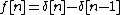 . A theorem stated above guarantees that the Fourier Karhunen–Loève basis produces a smaller expected approximation error than a canonical basis of Diracs
 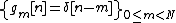 . Indeed, we do not know a priori the abscissa of the non-zero coefficients of Y, so there is no particular Dirac that is better adapted to perform the approximation. But the Fourier vectors cover the whole support of Y and thus absorb a part of the signal energy.
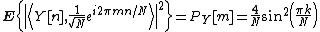
Selecting higher frequency Fourier coefficients yields a better mean-square approximation than choosing a priori a few Dirac vectors to perform the approximation. The situation is totally different for non-linear approximations. If  then the discrete Fourier basis is extremely inefficient because f and hence Y have an energy that is almost uniformly spread among all Fourier vectors. In contrast, since f has only two non-zero coefficients in the Dirac basis, a non-linear approximation of Y with {{math|M ≥ 2}} gives zero error.[6]
Principal component analysis
{{Main article|Principal component analysis}}We have established the Karhunen–Loève theorem and derived a few properties thereof. We also noted that one hurdle in its application was the numerical cost of determining the eigenvalues and eigenfunctions of its covariance operator through the Fredholm integral equation of the second kind
However, when applied to a discrete and finite process 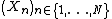 , the problem takes a much simpler form and standard algebra can be used to carry out the calculations.
Note that a continuous process can also be sampled at N points in time in order to reduce the problem to a finite version.
We henceforth consider a random N-dimensional vector 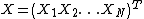 . As mentioned above, X could contain N samples of a signal but it can hold many more representations depending on the field of application. For instance it could be the answers to a survey or economic data in an econometrics analysis.
As in the continuous version, we assume that X is centered, otherwise we can let  (where
  is the mean vector of X) which is centered.
Let us adapt the procedure to the discrete case.
Covariance matrix
Recall that the main implication and difficulty of the KL transformation is computing the eigenvectors of the linear operator associated to the covariance function, which are given by the solutions to the integral equation written above.
Define Σ, the covariance matrix of X, as an N × N matrix whose elements are given by:

Rewriting the above integral equation to suit the discrete case, we observe that it turns into:

where 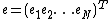 is an N-dimensional vector.
The integral equation thus reduces to a simple matrix eigenvalue problem, which explains why the PCA has such a broad domain of applications.
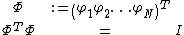
Since Σ is a positive definite symmetric matrix, it possesses a set of orthonormal eigenvectors forming a basis of  , and we write
  this set of eigenvalues and corresponding eigenvectors, listed in decreasing values of {{mvar|λi}}. Let also {{math|Φ}} be the orthonormal matrix consisting of these eigenvectors:
Principal component transform
It remains to perform the actual KL transformation, called the principal component transform in this case. Recall that the transform was found by expanding the process with respect to the basis spanned by the eigenvectors of the covariance function. In this case, we hence have:

In a more compact form, the principal component transform of X is defined by:
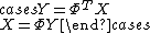
The i-th component of Y is  , the projection of X on
  and the inverse transform {{math|X {{=}} ΦY}} yields the expansion of {{mvar|X}} on the space spanned by the :

As in the continuous case, we may reduce the dimensionality of the problem by truncating the sum at some  such that

where α is the explained variance threshold we wish to set.
We can also reduce the dimensionality through the use of multilevel dominant eigenvector estimation (MDEE).[7]
Examples
The Wiener process
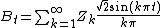
There are numerous equivalent characterizations of the Wiener process which is a mathematical formalization of Brownian motion. Here we regard it as the centered standard Gaussian process Wt with covariance function

We restrict the time domain to [a, b]=[0,1] without loss of generality.
The eigenvectors of the covariance kernel are easily determined. These are
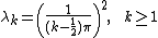
and the corresponding eigenvalues are

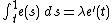
In order to find the eigenvalues and eigenvectors, we need to solve the integral equation:
differentiating once with respect to t yields:
a second differentiation produces the following differential equation:

The general solution of which has the form:
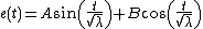
where A and B are two constants to be determined with the boundary conditions. Setting t = 0 in the initial integral equation gives e(0) = 0 which implies that B = 0 and similarly, setting t = 1 in the first differentiation yields e' (1) = 0, whence:

which in turn implies that eigenvalues of TKX are:
The corresponding eigenfunctions are thus of the form:
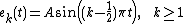
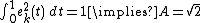
A is then chosen so as to normalize ek:
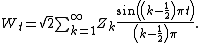
This gives the following representation of the Wiener process:
Theorem. There is a sequence {Zi}i of independent Gaussian random variables with mean zero and variance 1 such that
Note that this representation is only valid for  On larger intervals, the increments are not independent. As stated in the theorem, convergence is in the L2 norm and uniform in t.
The Brownian bridge
Similarly the Brownian bridge  which is a stochastic process with covariance function

can be represented as the series
Applications
{{Expand section|date=July 2010}}Adaptive optics systems sometimes use K–L functions to reconstruct wave-front phase information (Dai 1996, JOSA A).
Karhunen–Loève expansion is closely related to the Singular Value Decomposition. The latter has myriad applications in image processing, radar, seismology, and the like. If one has independent vector observations from a vector valued stochastic process then the left singular vectors are maximum likelihood estimates of the ensemble KL expansion.
Applications in signal estimation and detection
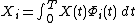
Detection of a known continuous signal S(t)
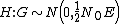
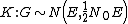
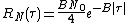
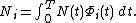
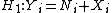
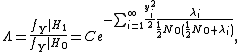
In communication, we usually have to decide whether a signal from a noisy channel contains valuable information. The following hypothesis testing is used for detecting continuous signal s(t) from channel output X(t), N(t) is the channel noise, which is usually assumed zero mean Gaussian process with correlation function 


Signal detection in white noise
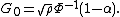
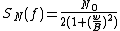
When the channel noise is white, its correlation function is
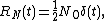
and it has constant power spectrum density. In physically practical channel, the noise power is finite, so:
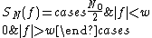
Then the noise correlation function is sinc function with zeros at  Since are uncorrelated and gaussian, they are independent. Thus we can take samples from X(t) with time spacing

Let  . We have a total of
  i.i.d observations
 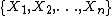 to develop the likelihood-ratio test. Define signal
  , the problem becomes,


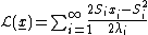
The log-likelihood ratio

As {{math|t → 0}}, let:
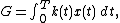
Then G is the test statistics and the Neyman–Pearson optimum detector is

As G is Gaussian, we can characterize it by finding its mean and variances. Then we get
where

is the signal energy.
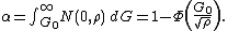
The false alarm error

And the probability of detection:

where Φ is the cdf of standard normal, or Gaussian, variable.
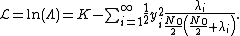
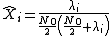
Signal detection in colored noise
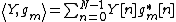
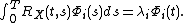
When N(t) is colored (correlated in time) Gaussian noise with zero mean and covariance function  we cannot sample independent discrete observations by evenly spacing the time. Instead, we can use K–L expansion to uncorrelate the noise process and get independent Gaussian observation 'samples'. The K–L expansion of N(t):
where  and the orthonormal bases
  are generated by kernel
  , i.e., solution to

Do the expansion:
where  , then
under H and  under K. Let
 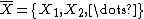 , we have
are independent Gaussian r.v's with variance
under H:are independent Gaussian r.v's.
under K:are independent Gaussian r.v's.

Hence, the log-LR is given by
and the optimum detector is

Define
then 
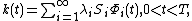
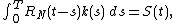
How to find k(t)
Since

k(t) is the solution to

If N(t)is wide-sense stationary,
which is known as the Wiener–Hopf equation. The equation can be solved by taking fourier transform, but not practically realizable since infinite spectrum needs spatial factorization. A special case which is easy to calculate k(t) is white Gaussian noise.

The corresponding impulse response is h(t) = k(T − t) = CS(T − t). Let C = 1, this is just the result we arrived at in previous section for detecting of signal in white noise.
Test threshold for Neyman–Pearson detector
Since X(t) is a Gaussian process,
is a Gaussian random variable that can be characterized by its mean and variance.

Hence, we obtain the distributions of H and K:


The false alarm error is
So the test threshold for the Neyman–Pearson optimum detector is
Its power of detection is

When the noise is white Gaussian process, the signal power is

Prewhitening
For some type of colored noise, a typical practise is to add a prewhitening filter before the matched filter to transform the colored noise into white noise. For example, N(t) is a wide-sense stationary colored noise with correlation function
The transfer function of prewhitening filter is

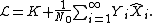
Detection of a Gaussian random signal in Additive white Gaussian noise (AWGN)
When the signal we want to detect from the noisy channel is also random, for example, a white Gaussian process X(t), we can still implement K–L expansion to get independent sequence of observation. In this case, the detection problem is described as follows:

X(t) is a random process with correlation function


The K–L expansion of X(t) is
where
and  are solutions to
So  's are independent sequence of r.v's with zero mean and variance
  . Expanding Y(t) and N(t) by , we get

where
As N(t) is Gaussian white noise, 's are i.i.d sequence of r.v with zero mean and variance  , then the problem is simplified as follows,

The Neyman–Pearson optimal test:
so the log-likelihood ratio is
Since
is just the minimum-mean-square estimate of given  's,
's,
K–L expansion has the following property: If

where

then

So let

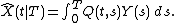
Noncausal filter Q(t,s) can be used to get the estimate through
By orthogonality principle, Q(t,s) satisfies

However, for practical reasons, it's necessary to further derive the causal filter h(t,s), where h(t,s) = 0 for s > t, to get estimate  . Specifically,

See also
- Principal component analysis
- Proper orthogonal decomposition
- Polynomial chaos
Notes
2. ^{{Citation |last=Ghoman |first=Satyajit |last2= Wang|first2= Zhicun|last3=Chen |first3=PC |last4=Kapania|first4=Rakesh|title= A POD-based Reduced Order Design Scheme for Shape Optimization of Air Vehicles|booktitle=Proc of 53rd AIAA/ASME/ASCE/AHS/ASC Structures, Structural Dynamics, and Materials Conference, AIAA-2012-1808, Honolulu, Hawaii |year=2012 }}
3. ^Karhunen–Loeve transform (KLT), Computer Image Processing and Analysis (E161) lectures, Harvey Mudd College
4. ^{{Citation |first=C.K. |last=Raju |title=Kosambi the Mathematician |journal=Economic and Political Weekly |volume=44 |year=2009 |issue=20 |pages=33–45 }}
5. ^{{Citation |first=D. D. |last=Kosambi |title=Statistics in Function Space |journal=Journal of the Indian Mathematical Society |volume=7 |year=1943 |issue= |pages=76–88 |mr=9816 }}.
6. ^A wavelet tour of signal processing-Stéphane Mallat
7. ^X. Tang, “Texture information in run-length matrices,” IEEE Transactions on Image Processing, vol. 7, No. 11, pp. 1602–1609, Nov. 1998
References
- {{cite book
|first1=Henry
|last1=Stark
|first2=John W.
|last2=Woods
|title=Probability, Random Processes, and Estimation Theory for Engineers
|publisher=Prentice-Hall, Inc
|year=1986
|isbn=978-0-13-711706-2
|url = http://openlibrary.org/books/OL21138080M/Probability_random_processes_and_estimation_theory_for_engineers
}}
- {{cite book
|first1=Roger
|last1=Ghanem
|first2=Pol
|last2=Spanos
|publisher = Springer-Verlag
|isbn = 978-0-387-97456-9
|title = Stochastic finite elements: a spectral approach
|url = http://openlibrary.org/books/OL1865197M/Stochastic_finite_elements
|year = 1991
}}
- {{cite book
|first1=I.
|last1=Guikhman
|first2=A.
|last2=Skorokhod
|title=Introduction a la Théorie des Processus Aléatoires
|publisher=Éditions MIR
|year=1977
}}
- {{cite book
|first1=B.
|last1=Simon
|title=Functional Integration and Quantum Physics
|publisher=Academic Press
|year=1979
}}
- {{cite journal
|last1=Karhunen
|first1=Kari
|title=Über lineare Methoden in der Wahrscheinlichkeitsrechnung
|journal=Ann. Acad. Sci. Fennicae. Ser. A. I. Math.-Phys.
|year=1947
|volume=37
|pages=1–79
}}
- {{cite book
|first1=M.
|last1=Loève
|title=Probability theory. Vol. II, 4th ed.
|series=Graduate Texts in Mathematics
|volume=46
|publisher=Springer-Verlag
|year=1978
|isbn=978-0-387-90262-3
}}
- {{cite journal
|first1=G.
|last1=Dai
|title=Modal wave-front reconstruction with Zernike polynomials and Karhunen–Loeve functions
|journal=JOSA A
|volume=13
|issue=6
|page=1218
|year=1996
|doi=10.1364/JOSAA.13.001218
|bibcode=1996JOSAA..13.1218D
}}
- Wu B., Zhu J., Najm F.(2005) "A Non-parametric Approach for Dynamic Range Estimation of Nonlinear Systems". In Proceedings of Design Automation Conference(841-844) 2005
- Wu B., Zhu J., Najm F.(2006) "Dynamic Range Estimation". IEEE Transactions on Computer-Aided Design of Integrated Circuits and Systems, Vol. 25 Issue:9 (1618–1636) 2006
- {{cite journal
|title=Entropy Encoding, Hilbert Space and Karhunen–Loeve Transforms
|first1=Palle E. T.
|last1=Jorgensen
|first2=Myung-Sin
|last2=Song
|arxiv=math-ph/0701056
|year=2007
|doi=10.1063/1.2793569
|volume=48
|issue=10
|journal=Journal of Mathematical Physics
|page=103503
|bibcode=2007JMP....48j3503J
}}
External links
- Mathematica KarhunenLoeveDecomposition function.
- E161: Computer Image Processing and Analysis notes by Pr. Ruye Wang at Harvey Mudd College
- Jenny Hagel
- Jenny Haglund
- Jenny Harper
- Jenny Harragon
- Jenny Herz
- Jenny Higham
- Jenny Hill (judoka)
- Jenny Hoad
- Jenny Hoffman
- Jenny Hoppe
- Jenny Hunter Groat
- Jenny Hyslop
- Jenny James
- Jenny James (orienteer)
- Jenny James (orienteering)
- Jenny Jenkins
- Jenny Jenny
- Jenny Jones (Green politician)
- Jenny Jones (politician)
- Jenny Jonsson
- Jenny Jordan
- Jenny Juggs
- Jenny Jump (disambiguation)
- Jenny Karin Olsson
- Jenny Karlsson